Update on Assessment (i) PT2 (ii) P3 (iii) EOY

(1) Performance Task 2

This constitutes the Elementary Mathematics component of Assessment.

The performance task focuses on the topic of Geometrical Proof - Circle Properties. (please refer to Blog entry on Mathematics Performance Task 2)

Deadline for submission is Term 4 Week 1 (first lesson)

(2) Paper 3

This constitutes the Additional Mathematics component of Assessment.

This will be conducted in Term 4.

Students are expected to familiarise themselves with GC-TI84+.

(please refer to your Math teacher on information on use of GC-TI84+)

(3) End-of-Year Examination: Mathematics

Information pertaining to the Maths exam has been communicated to the students in the GoogleSite (as well as the Maths blog).

Elementary Mathematics paper 1

Date: 27 September 2013 (Friday)

Duration: 1 hour 30 minutes

Elementary Mathematics paper 2

Date: 30 September 2013 (Monday)

Duration: 2 hours

Additional Mathematics

Date: 4 October 2013 (Friday)

Duration: 2 hours 30 minutes

Table of Specification

A. Elementary Mathematics

•   Numbers and the four operations (moe 1.1)

•   Percentage (moe 1.3)

•   Kinematics / speed  (moe 1.4)

•   Algebraic representation and formulae (moe 1.5)

•   Functions and graphs (moe 1.7)

•   Algebraic manipulation (moe 1.6)

•   Solutions of equations and inequalities (moe 1.8)

•   Congruence and similarity (moe 2.2)

•   Properties of circles (moe 2.3)

•   Coordinate geometry (moe 2.6)

•   Data analysis  (moe 3.2)

B. Additional Mathematics

(A1) Equations and inequalities 

       Conditions for a quadratic equation

       Solving simultaneous equations in two variables with at least one linear 
equation, by substitution

       Relationships between the roots and coefficients of a quadratic equation

       Solving quadratic inequalities, and representing the solution on the number line

(A2) Indices and surds

       Four operations on indices and surds, including rationalising the denominator

       Solving equations involving indices and surds

(A3) Polynomials and Partial Fractions

       Multiplication and division of polynomials

       Use of remainder and factor theorems

       Factorisation of polynomials

       Partial fractions

(A4) Binomial Expansions

(A5) Power, Exponential, Logarithmic, and Modulus functions

(G1)  Trigonometric functions, identities and equations.

• ·       Six trigonometric functions for angles of any magnitude (in degrees or radians)
• ·       Principal values of sin–1x, cos–1x, tan–1x
• ·       Exact values of the trigonometric functions for special angles  
(30°,45°,60°) or (π/6,  π/4,  π/3)
• ·       Amplitude, periodicity and symmetries related to the sine and cosine functions 

• ·       Graphs of y  = asin(bx) ,     y  = a sin(x/b + c),    y  = acos(bx) ,     y  = a cos(x/b + c) and         y  = atan(bx) , where a is real, b is a positive integer and c is an integer.
• ·       Use of the following
• ∗   (BASIC TRIG RULES)
•      sin A/cos A=tan A,
•      cos A/sin A=cot A,    
•      sin2A+cos2A=1,
•      sec2A=1+tan2A,
•      cosec2A =1+cot2A
•      (DOUBLE ANLES)
•      the expansions of sin(A ± B), cos(A ± B)  and tan(A ± B)
•      the formulae for sin 2A, cos 2A and tan 2A
•      (R-FORMULA) - the expression for acosu +  bsinu in the form Rcos(u ± a) or R sin (u ± a)
•      Simplification of trigonometric expressions
• ·    Solution of simple trigonometric equations in a given interval (excluding 
general solution)
• ·    Proofs of simple trigonometric identities

(G2) Coordinate Geometry

       Condition for two lines to be parallel or perpendicular

(G2) Linear Law

       Transformation of given relationships, including   y = axn and y = kbx, to linear form to determine the unknown constants from a straight line graph

Resource and References

The following would be useful for revision:

• Maths Workbook
• Study notes
• Homework Handouts
• Exam Prep Booklets (that was given since the beginning of the year)
• Ace Learning Portal - where they could attempt practices that are auto-mark
• Past GCEO EM and AM questions (students were recommended to purchase these at the beginning of the year)

(4) General Consultation and Timed-trial during the school holidays

During the school holidays, there would be a timed-trial on Monday 9 September 2013 (Monday). The focus would be on Additional Mathematics and students are strongly encouraged to attend.

Duration: 0800 - 1030 (2 hours 30 minutes) 

Mathematics Performance Task 2

Due Term 4 Week 1 (first Mathematics Lesson)

the file could be downloaded from google site.

Please fill-up this form once you have submitted the work.

4. Uses of Binomial Theorem

Uses
-  It is used in statistics to calculate the binomial distribution.(Probability distribution is the probability        distribution of the number of successes in a sequence of n independent in yes/no distribution)
- This allows statisticians to determine the probability of a given number of favorable outcomes in a          repeated number of trials.
- Binomial expansion is also interesting from a mathematical point of view--it gives mathematicians insight into the properties of polynomials.
- Used in the distribution of IP addresses

Conceptual aspects
-This is the formula.

The way to derive the expanded form of a binomial with a exponential e.g. 4.

Lets just have the binomial be (a+b)

(a+b)^3 = a^3 + 3(a^2)b + 3ab^2 + b^3

As can be seen, the a exponents go from 3 to 0. (a^3, 3(a^2)b, 3ab^2,  b^3)

The b exponents go from 0 to 3. (a^3, 3(a^2)b, 3ab^2, b^3)

The coefficients go 1,3,3,1 (3rd row of the Pascal triangle)

To get the coefficients, you can use the above formula. Factorial = !

k is the order of the terms (e.g. 2nd or 3rd term)

e.g. to get the coefficient of the 42nd term of a binomial to the power of 50 e.g. ( a+b )^50

50! / (42!)(50-42)! = 536878650

You can get the coefficient of any term using this formula. Used together with the pattern of the exponents of the a and b terms, you can get the expanded form. ( faster than expanding). It is still very slow.

Below is an example of how to use the formula for binomial expansion to get the expanded form of the binomial cubed.

How is it used in probability?

Pascal's Triangle

Pascal's Triangle

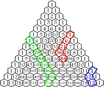
At the tip of Pascal's Triangle is the number 1, which makes up the zeroth row. The first row (1 & 1) contains two 1's, both formed by adding the two numbers above them to the left and the right, in this case 1 and 0 (all numbers outside the Triangle are 0's). Do the same to create the 2nd row: 0+1=1; 1+1=2; 1+0=1. And the third: 0+1=1; 1+2=3; 2+1=3; 1+0=1. In this way, the rows of the triangle go on infinitely. A number in the triangle can also be found by nCr (n Choose r) where n is the number of the row and r is the element in that row. For example, in row 3, 1 is the zeroth element, 3 is element number 1, the next three is the 2nd element, and the last 1 is the 3rd element. The formula for nCr is:

n!

--------

r!(n-r)!

! means factorial, or the preceeding number multiplied by all the positive integers that are smaller than the number. 5! = 5 × 4 × 3 × 2 × 1 = 120

The Sums of the Rows:

Sum of  numbers in any row is equal to 2 to the n^th power or 2ⁿ, when n is the number of the row. For example:

2⁰ = 1

2¹ = 1+1 = 2

2² = 1+2+1 = 4

2³ = 1+3+3+1 = 8

2⁴ = 1+4+6+4+1 = 16

Prime Numbers

If the 1^st element in a row is a prime number

Hockey Stick Pattern:

Diagonal of numbers of any length is selected starting at any of the 1's bordering the sides of the triangle and ending on any number inside the triangle on that diagonal, the sum of the numbers inside the selection is equal to the number below the end of the selection that is not on the same diagonal itself

1+6+21+56 = 84
1+7+28+84+210+462+924 = 1716
1+12 = 13

Fibonnacci's Sequence:

Fibonnacci's Sequence can also be located in Pascal's Triangle. The sum of the numbers in the consecutive rows shown in the diagram are the first numbers of the Fibonnacci Sequence. The Sequence can also be formed in a more direct way, very similar to the method used to form the Triangle, by adding two consecutive numbers in the sequence to produce the next number. The creates the sequence: 1,1,2,3,5,8,13,21,34, 55,89,144,233, etc . . . . The Fibonnacci Sequence can be found in the Golden Rectangle, the lengths of the segments of a pentagram, and in nature, and it decribes a curve which can be found in string instruments, such as the curve of a grand piano.

Hao Xian, Balram, Darryl lam, Enoch, Hao en.

Pascal Triangle and its relationship between Fibonacci Sequence and Binomial Expansion

Who is Pascal?

Blaise Pascal (19 June 1623 – 19 August 1662) was a French mathematician, physicist, inventor, writer and Christian philosopher. He was a child prodigy who was educated by his father, a tax collector in Rouen. Pascal's earliest work was in the natural and applied sciences where he made important contributions to the study of fluids, and clarified the concepts of pressure and vacuum by generalizing the work of Evangelista Torricelli (who was the creator of the barometer). Pascal also wrote in defense of the scientific method.

His notable contributions:

Pascal's Wager

Pascal's triangle

Pascal's law

Pascal's theorem

DID YOU KNOW: He gave up work in maths in 1654 due to a religious experience (He was a Roman Catholic)

Pascal Triangle

Relationship between Pascal Triangle and Fibonacci Sequence

The squares adjacent to each other can be used to derive the Fibonacci sequence.

Each line is x2 of the earlier line (Besides line one)

The relationship between the Pascal Triangle and Binomial Expansion

Done by: Charlene, Dylaine, Esther, Jemaimah, Aziel and Dawn

Binomial Theorem - Question 3

WHAT IS BINOMIAL THEOREM?

The expansion of 2 variables to a certain power >0 made simpler with pascals triangle.

Using pascal's triangle to do binomial expansion.

-Each expansion is polynomial.

Some of the patterns observed from the expansion.

1. There is one more term than the power of the exponent, n, when the expression is expanded. there are terms in the expansion of (a + b)ⁿ.

2. In each term, the sum of the exponents is n, the power to which the binomial is raised.

3. The exponents of a start with n, the power of the binomial, and decrease to 0. The last term has no factor of a. The first term has no factor of b, so powers of b start with 0 and increase to n.

4. The coefficients start at 1 and increase through certain values about "half"-way and then decrease through these same values back to 1.

These patterns can be quantified and put into a formula:

IS THERE A POLYNOMIAL THEOREM?

Yes there is.

The polynomial theorem here is referring to the remainder and factor theorem we learnt before.

BINOMIAL THEOREM AND PASCAL'S TRIANGLE.

Compare the below 2 diagrams. Notice any similarities?

Look at the coefficients of the variables in the first diagram. Then, compare them to the numbers of the pascal's triangle. Those that are in the same row have the same coefficients.

Thus, the binomial theorem is related to the pascal's triangle by its coefficients.

Lesson Summary 22/8 - R Formula

Introduction: Graphical method

Graphs of 5sinθ + 2cosθ and sqrt(29)sin(θ+21.8º)

The graph of sqrt(29)sin(θ+21.8º) is an approximation, and thus is slightly out of phase with the graph of 5 sin θ + 2 cos θ. However, when drawn, the 2 graphs are almost the same, which reflects that the functions 5sinθ + 2cosθ and sqrt(29)sin(θ+21.8º) are identical.

Graph of 5sinθ and graph of 2cosθ

Finding Ymin and Ymax of the functions from the graph:

The Ymax and Ymin values of 5sinθ + 2cosθ and sqrt(29)sin(θ+21.8º) are not the Ymax and Ymin values of 5sinθ and 2cosθ added together.

Graph of 5sinθ + 2cosθ plotted with the graphs of 5sinθ and 2cosθ

Algebraic Method:

Solving 5sinθ + 2cosθ =0:

Solving 5sinθ + 2cosθ by expressing in the form Rsin(θ+α), to find the ymin and ymax:

TRIGONOMETRY - Compound and Double Angle

Trigonometry T1-84 (Activity)

his activity is walks you through the steps to perform sine regression for a randomly generated data set using the TI-84.

Step 1: Get a TI-84 Graphing Calculator (or similar).

• Don’t have one? If you use Windows, you can download the attached Emulator (ZIP file), extract the Zip folder, and run the Wabbitemu.exe file. Load the rom file when prompted and just choose the View > Enable skin option to work with your virtual calculator.

Step 2: Get some data.

• Go to the Randomized Wave Data Generator and use the form to get some randomly-generated data (check the boxes for more interesting data).
• Your data should be different from every other data set on earth, so copy and paste it to a (spreadsheet or word-processor) file for your later use.

Step 3: Enter the Data into your Calculator.

1. Press Y= and clear the Y1 function.
2. Press STATPLOT (2nd followed by Y=) and choose Plot1.
3. Under Plot1, select On (press ENTER), after Type select the drawing of disconnected dots, and make sure you have Xlist: L1(2nd followed by 1) and Ylist: L2 (2nd followed by 2).
4. Press STAT. With EDIT highlighted, select 1:Edit…
5. In the table that appears, under L1 type the x values and under L2 type the values of y. Make sure your L1 and L2 lists have the same length.
6. Press ZOOM and choose option 9:ZoomStat to look at a scatter plot of your data.

Step 4: Find the Sine Wave of Best Fit for the Data.

1. Press STAT. Press the right arrow key to highlight CALC. Then scroll down to select C:SinReg and pressENTER ONCE.
2. [Older Versions] After the word SinReg, which should now be on the screen, enter L1(2nd followed by 1), then type a comma (just above the 7 key), then enter L2 (2nd followed by 2), then type another comma, and then enter Y1 (press VARS, then select Y-VARS , then select FUNCTION, and then select Y1) . Your screen should now read SinReg L1, L2, Y1. Then press ENTER ONCE.
3. [Newer Versions] In the SinReg screen, choose Iterations:3 Xlist:L1, Ylist:L2 and Store RegEq: Y1 (press VARS, then select Y-VARS , then select FUNCTION, and then select Y1). Then highlight Calculate and press ENTER ONCE.
4. The calculator should now display the values for a, b, c, and d in the function f(x)=asin(bx+c)+dthat best fits the given data set.
5. Press GRAPH to see the sine regression function plotted along with your scatter plot and press Y1 to see the equation of your wave.